

4. Asymptotic Approximations
This chapter examines methods of deriving
approximate solutions to problems or of approximating exact solutions,
which allow us to develop concise and precise
estimates of quantities of interest when analyzing algorithms.
4.1 Notation for Asymptotic Approximations
The following notations, which date back at least to the beginning of the century, are widely used for making precise statements about the approximate value of functions:Definition. Given a function $f(N)$, we write
- $g(N)=O(f(N))$ if and only if $|g(N)/f(N)|$ is bounded from above as $N\to\infty$
- $g(N)=o(f(N))$ if and only if $g(N)/f(N)\to 0$ as $N\to\infty$
- $g(N)\sim f(N)$ if and only if $g(N)/f(N)\to 1$ as $N\to\infty$.
The $O$- and $o$-notations provide ways to express upper bounds (with $o$ being the stronger assertion), and the $\sim$-notation provides a way to express asymptotic equivalence.
In the analysis of algorithms, we avoid direct usages such as “the average value of this quantity is $O{f(N)}$” because this gives scant information for the purpose of predicting performance. Instead, we strive to use the $O$-notation to bound “error” terms that have far smaller values than the main, or “leading” term. Informally, we expect that the terms involved should be so small as to be negligible for large $N$.
$O$-approximations. We say that $g(N)=f(N)+O(h(N))$ to indicate that we can approximate $g(N)$ by calculating $f(N)$ and that the error will be within a constant factor of $h(N)$. As usual with the $O$-notation, the constant involved is unspecified, but the assumption that it is not large is often justified. As discussed below, we normally use this notation with $h(N)=o(f(N))$.
$o$-approximations. A stronger statement is to say that $g(N)=f(N)+o(h(N))$ to indicate that we can approximate $g(N)$ by calculating $f(N)$ and that the error will get smaller and smaller compared to $h(N)$ as $N$ gets larger. An unspecified function is involved in the rate of decrease, but the assumption that it is never large numerically (even for small $N$) is often justified.
$\sim$-approximations. The notation $g(N)\sim f(N)$ is used to express the weakest nontrivial $o$-approximation $g(N)=f(N)+o(f(N))$.
These notations are useful because they can allow suppression of unimportant details without loss of mathematical rigor or precise results. If a more accurate answer is desired, one can be obtained, but most of the detailed calculations are suppressed otherwise. We will be most interested in methods that allow us to keep this “potential accuracy,” producing answers that could be calculated to arbitrarily fine precision if desired.
Asymptotics of linear recurrences. Linear recurrences provide an illustration of the utility of asymptotics. Any linear recurrent sequence $\{a_n\}$ has a rational OGF and is a linear combination of terms of the form $\beta^{n}n^{j}$. Asymptotically speaking, only a few terms need be considered, because those with larger $\beta$ exponentially dominate those with smaller $\beta$. For example, exact solution to $$a_n=5a_{n-1}-6a_{n-2}\qquad\hbox{for $n>1$ with $a_0=0$ and $a_1=1$}$$ is $3^n-2^n$, but the approximate solution $3^n$ is accurate to within a thousandth of a percent for $n>25$. We need keep track only of terms associated with the largest absolute value or modulus.
Theorem 4.1 (Asymptotics for linear recurrences). Assume that a rational generating function $f(z)/g(z)$, with $f(z)$ and $g(z)$ relatively prime and $g(0)\ne0$, has a unique pole $1/\beta$ of smallest modulus (that is, $g(1/\alpha)=0$ and $\alpha\ne\beta$ implies that $|1/\alpha|>|1/\beta|$, or $|\alpha|<|\beta|$). Then, if the multiplicity of $1/\beta$ is $\nu$, we have $$[z^n]{f(z)\over g(z)}\sim C\beta^{n}n^{\nu-1}\quad\hbox{where}\quad C=\nu{(-\beta)^\nu f(1/\beta)\over g^{(\nu)}(1/\beta)}.$$
4.2 Asymptotic Expansions.
We prefer the equation $f(N)=c_0g_0(N)+O(g_1(N))$ with $g_1(N)=o(g_0(N))$ to the equation $f(N)=O(g_0(N))$ because it provides the constant $c_0$, and therefore allows us to provide specific estimates for $f(N)$ that improve in accuracy as $N$ gets large.The concept of an asymptotic expansion, developed by Poincaré, generalizes this notion:
Definition. Given a sequence of functions $\{g_k(N)\}_{k\ge0}$ with $g_{k+1}(N)=o(g_k(N))$ for $k\ge0$, $$f(N)\sim c_0g_0(N)+c_1g_1(N)+c_2g_2(N)+\ldots$$ is called an asymptotic series for $f$, or an asymptotic expansion of $f$. The asymptotic series represents the collection of formulae $$\eqalign{ f(N)&=O(g_0(N))\cr f(N)&=c_0g_0(N)+O(g_1(N))\cr f(N)&=c_0g_0(N)+c_1g_1(N)+O(g_2(N))\cr f(N)&=c_0g_0(N)+c_1g_1(N)+c_2g_2(N)+O(g_3(N))\cr &\hskip5pt\vdots\cr}$$ and the $g_k(N)$ are referred to as an asymptotic scale.
This general approach allows asymptotic expansions to be expressed in terms of any infinite series of functions that decrease (in a $o$-notation sense). However, we are most often interested in a very restricted set of functions: indeed, we are very often able to express approximations in terms of decreasing powers of $N$ when approximating functions as $N$ increases. Other functions occasionally are needed, but we normally will be content with an asymptotic scale consisting of terms of decreasing series of products of powers of $N$, $\log N$, iterated logarithms such as $\log\log N$, and exponentials.
Each additional term that we take from the asymptotic series gives a more accurate asymptotic estimate. Full asymptotic series are available for many functions commonly encountered in the analysis of algorithms, and we primarily consider methods that could be extended, in principle, to provide asymptotic expansions describing quantities of interest. We can use the $\sim$-notation to simply drop information on error terms or we can use the $O$-notation or the $o$-notation to provide more specific information.
This table gives classic asymptotic expansions for four basic functions, derived from truncating Taylor series. Other similar expansions follow immediately from the generating functions given in Chapter 3. In the sections that follow, we describe methods of manipulating asymptotic series using these expansions.
| function | asymptotic expansion |
|---|---|
| exponential | $\displaystyle e^x=1+x+{x^2\over2}+{x^3\over6}+O(x^4)$ |
| logarithmic | $\displaystyle\ln(1+x)=x-{x^2\over2}+{x^3\over3}+O(x^4)$ |
| binomial | $\displaystyle(1+x)^k=1+kx+{k\choose2}x^2+{k\choose3}x^3+O(x^4)$ |
| geometric | $\displaystyle{1\over1-x}=1+x+x^2+x^3+O(x^4)$ |
Example.
To expand $\ln(N-2)$ for $N\to\infty$, pull out the leading term, writing
$$\ln(N-2) = \ln N + \ln(1-{2\over N}) = \ln N - {2\over N} +O({1\over N^2}).$$
That is, we use the substitution ($x = -2/N$)
with $x\to0$.
Nonconvergent asymptotic series. Any convergent series leads to a full asymptotic approximation, but it is very important to note that the converse is not true---an asymptotic series may well be divergent. For example, we might have a function $$f(N)\sim\sum_{k\ge0}{k!\over N^k}$$ implying (for example) that $$f(N)=1+{1\over N}+{2\over N^2}+{6\over N^3}+O({1\over N^4})$$ even though the infinite sum does not converge. Why is this allowed? If we take any fixed number of terms from the expansion, then the equality implied from the definition is meaningful, as $N\to\infty$. That is, we have an infinite collection of better and better approximations, but the point at which they start giving useful information gets larger and larger.
This table gives asymptotic series for special number sequences that are encountered frequently in combinatorics and the analysis of algorithms. We consider many of these expansions later as examples of manipulating and deriving asymptotic series. We refer to them frequently later in the book because the number sequences themselves arise naturally when studying properties of algorithms.
| function | asymptotic expansion |
|---|---|
| factorial (Stirling's formula) | $\displaystyle N!=\sqrt{2\pi N}\Bigl({N\over e}\Bigr)^N\Bigl(1+{1\over12N}+{1\over288N^2}+O({1\over N^3})\Bigr)$ |
| log version of Stirling's formula | $\qquad\displaystyle \ln N!=\Bigl(N+{1\over2}\Bigr)\ln N -N + \ln\sqrt{2\pi}+{1\over 12N}+O({1\over N^3})\qquad$ |
| harmonic numbers | $\displaystyle H_N=\ln N + \gamma + {1\over2N} -{1\over12N^2}+O({1\over N^4})$ |
| binomial coefficients | $\displaystyle {N\choose k}={N^k\over k!}\Bigl(1+O({1\over N})\Bigr)\quad{\rm for\ }k=O(1)$ |
| binomial coefficients (center) | $\displaystyle {N\choose k}={2^N\over\sqrt{\pi N/2}}\Bigl(1+O({1\over N})\Bigr)\quad\hbox{for\ }k={N\over2}+O(1)$ |
| normal approximation to the binomial distribution | $\displaystyle {2N\choose N- k}{1\over 2^{2N}}={e^{-{k^2/N}}\over\sqrt{\pi N}} + O({1\over N^{3/2}})$ |
| Poisson approximation to the binomial distribution | $\displaystyle{N\choose k}p^k(1-p)^{N-k}={\lambda^ke^{-\lambda}\over k!}+o(1)\quad{\rm for\ }p = \lambda/N$ |
| Stirling numbers of the first kind | $\displaystyle {N\brack k}\sim{(N-1)!\over (k-1)!}(\ln N)^{k-1} \quad{\rm for\ } k = O(1)$ |
| Stirling numbers of the second kind | $\displaystyle {N\brace k}\sim{k^N\over k!}\quad{\rm for\ } k = O(1)$ |
| Bernoulli numbers | $\displaystyle B_{2N}=(-1)^{N}{(2N)!\over(2\pi)^{2N}}(-2+O(4^{-N}))$ |
| Catalan numbers | $\displaystyle T_N\equiv{1\over N+1}{2N\choose N}={4^N\over\sqrt{\pi N^3}}\Bigl(1 + O({1\over N})\Bigr)$ |
| Fibonacci numbers | $\displaystyle F_N={\phi^N\over\sqrt5}+O({\phi^{-N}}) \quad{\rm where\ }\phi={1+\sqrt5\over2}$ |
4.3 Manipulating Asymptotic Expansions
The manipulation of asymptotic expansions generally reduces in a straightforward manner to the application of one of several basic operations, which we consider in turn. In the examples, we will normally consider series with one, two, or three terms (not counting the $O$-term). Of course, the methods apply to longer series, as well.Simplification. An asymptotic series is only as good as its $O$-term, so anything smaller (in an asymptotic sense) may as well be discarded. For example, the expression $\ln N + O(1)$ is mathematically equivalent to the expression $\ln N + \gamma + O(1)$, but simpler.
Substitution. The simplest and most common asymptotic series derive from substituting appropriately chosen variable values into Taylor series expansions or into other asymptotic series. For example, by taking $x=-1/N$ in the geometric series $${1\over 1-x}=1+x+x^2+O({x^3})\qquad\hbox{as $x\to0$}$$ gives $${1\over N+1}={1\over N}-{1\over N^2}+ O({1\over N^3})\qquad\hbox{as $N\to\infty$}.$$ Similarly, $$e^{1/N}= 1+{1\over N}+{1\over 2N^2}+{1\over 6N^3}+\cdots+ {1\over k!N^k} + O({1\over N^{k+1}}).$$
Factoring. When the “approximate” value of a function is obvious upon inspection it is worthwhile to rewrite the function making this explicit in terms of relative or absolute error. For example, the function $1/(N^2+N)$ is obviously very close to $1/N^2$ for large $N$, which we can express explicitly by writing $$\eqalign{{1\over N^2+N}&={1\over N^2}{1\over 1+1/N}\cr &={1\over N^2}\Bigl(1+{1\over N}+O({1\over N^2})\Bigr)\cr &={1\over N^2}+{1\over N^3}+O({1\over N^4}).\cr}$$ When the approximate value is not immediately obvious, a short trial-and-error process might be necessary.
Multiplication. Multiplying two asymptotic series is simply a matter of doing the term-by-term multiplications, then collecting terms. For example, $$\eqalign{ (H_N)^2&=\Bigl(\ln N+\gamma+ O({1\over N})\Bigr) \Bigl(\ln N+\gamma+O({1\over N})\Bigr)\cr &=\Bigl((\ln N)^2+\gamma\ln N+O({\log N\over N})\Bigr)\cr &\qquad+\Bigl(\gamma\ln N+\gamma^2+O({1\over N})\Bigr)\cr &\qquad+\Bigl(O({\log N\over N})+O({1\over N})+O({1\over N^2})\Bigr)\cr &=(\ln N)^2+2\gamma\ln N+\gamma^2+O({\log N\over N}).\cr}$$
In this case, the product has less absolute asymptotic accuracy than the factors—the result is only accurate to within $O({\log N/N})$. This is normal, and we typically need to begin a derivation with asymptotic expansions that have more terms than desired in the result. Often, we use a two-step process: do the calculation, and if the answer does not have the desired accuracy, express the original components more accurately and repeat the calculation.
Division. To compute the quotient of two asymptotic series, we typically factor and rewrite the denominator in the form $1/(1-x)$ for some symbolic expression $x$ that tends to 0, then expand as a geometric series, and multiply. For example, to compute an asymptotic expansion of $\tan x$, we can divide the series for $\sin x$ by the series for $\cos x$, as follows: $$\eqalign{ \tan x = {\sin x\over\cos x} &= {x - x^3/6 +O({x^5})\over 1 - x^2/2 +O({x^4})}\cr &= \Bigl(x - x^3/6 +O({x^5})\Bigr){1\over 1 - x^2/2 +O({x^4})}\cr &= \Bigl(x - x^3/6 +O({x^5})\Bigr)({1 + x^2/2 +O({x^4})})\cr &= x + x^3/3 +O({x^5}).\cr }$$
Exponentiation/logarithm. Writing $f(x)$ as $\exp\{\ln(f(x))\}$ is often a convenient start for doing asymptotics involving powers or products. A standard example is the following approximation for $e$: $$\eqalign{ \Bigl(1+{1\over N}\Bigr)^N &= \exp\Bigl\{N\ln\Bigl(1 + {1\over N}\Bigr)\Bigr\}\cr &= \exp\Bigl\{N\Bigl({1\over N} + O({1\over N^2}) \Bigr)\Bigr\} \cr &= \exp\Bigl\{1 + O({1\over N})\Bigr\}\cr &= e + O({1\over N}).\cr }$$
4.4 Asymptotic Approximations of Finite Sums
Frequently, we are able to express a quantity as a finite sum, and therefore we need to be able to accurately estimate the value of the sum. Some sums can be evaluated exactly. In many more cases, exact values are not available, or we may only have estimates for the quantities themselves being summed.Bounding the tail. When the terms in a finite sum are rapidly decreasing, an asymptotic estimate can be developed by approximating the sum with an infinite sum and developing a bound on the size of the infinite tail.
Example (derangements).$$N!\sum_{0\le k\le N}{(-1)^k\over k!} = N!e^{-1} - R_N \quad\hbox{where}\quad R_N= N!\sum_{k>N}{(-1)^k\over k!}.$$ Bound the tail $R_N$ by bounding the individual terms: $$|R_N|<{1\over N+1}+{1\over (N+1)^2}+{1\over (N+1)^3}+\ldots = {1\over N}.$$ Therefore, the sum is $N!e^{-1}+O({1/N})$. The convergence is so rapid that it is possible to show that the value is always equal to $N!e^{-1}$ rounded to the nearest integer.
Example (tries).$$\sum_{1\le k\le N}{1\over 2^k-1} = \sum_{k\ge 1}{1\over 2^k-1} - R_N, \quad\hbox{where}\quad R_N=\sum_{k>N}{1\over 2^k-1}.$$ The constant $1 + 1/3 + 1/7 + 1/15 + \ldots = 1.6066\cdots$ is an extremely good approximation to the finite sum (that is trivial to calculate to any reasonable desired accuracy) because $R_N < \sum_{k>N}{1/2^{k-1}}=1/2^{N-1}.$
Using the tail. When the terms in a finite sum are rapidly increasing, the last term often suffices to give a good asymptotic estimate for the whole sum.
Example.$$\sum_{0\le k\le N} k! = N!\Bigl(1+{1\over N}+\sum_{0\le k\le N-2}{k!\over N!}\ \Bigr) = N!\Bigl(1+O({1\over N})\Bigr),$$ since there are $N-1$ terms in the sum, each less than $1/(N(N-1))$.
Approximating sums with integrals. What is the magnitude of the error made when we use $$\int_a^b {f(x)}dx\quad\hbox{to estimate}\quad\sum_{a\le k < b} {f(k)}?$$ The answer to this question depends on the “smoothness” of the function $f(x)$. In each of the $b-a$ unit intervals between $a$ and $b$, we are using $f(k)$ to estimate $f(x)$. Letting $\delta_k = \max_{k\le x < k+1}|f(x)-f(k)|$ denote the maximum error in each interval, we can get a rough approximation to the total error: $$\sum_{a\le k < b} {f(k)}=\int_a^b {f(x)}dx + \Delta, \qquad\hbox{with\ }|\Delta|\le\sum_{a\le k < b}\delta_k.$$ If the function is monotone increasing or decreasing over the whole interval $[a,\/b]$, then the error term telescopes to simply $\Delta \le |f(a)-f(b)|$.
Example (Harmonic numbers).$$H_N=\sum_{1\le k\le N}{1\over k} = \int_1^N{1\over x}dx + \Delta = \ln N + \Delta$$ with $|\Delta| \le 1-1/N$, an easy proof that $H_N\sim\ln N$.
Example (Stirling's approximation (logarithmic form)).$$\ln N!=\sum_{1\le k\le N}{\ln k}= \int_1^N{\ln x}\,dx + \Delta = N\ln N - N +1+ \Delta$$ with $|\Delta|\le\ln N$, an easy proof that $\ln N!\sim N\ln N - N$.
More precise estimates of the error terms depend on the derivatives of the function. That is the topic of the next section.
4.5 Euler-Maclaurin Summation.
One of the most powerful tools in asymptotic analysis dates to the 18th century and enables us to approximate sums with integrals in two distinct ways.- A function is defined on a fixed interval and we evaluate a sum corresponding to sampling the function at an increasing number of points along the interval, with smaller and smaller step sizes, with the difference between the sum and the integral converging to zero (as in classic Reimann integration).
- The step size is fixed, so the interval of integration gets larger and larger, with the difference between the sum and the integral converging to a constant.
Theorem 4.2 (Euler-Maclaurin summation formula, first form). Let $f(x)$ be a function defined on an interval $[\,a,\,b\,]$ with $a$ and $b$ integers, and suppose that the derivatives $f^{(i)}(x)$ exist and are continuous for $1\le i\le 2m$, where $m$ is a fixed constant. Then $$\sum_{a\le k\le b} {f(k)} = \int_a^b {f(x)}dx +{f(a)+f(b)\over2} +\sum_{1\le i\le m}{B_{2i} \over (2i)!} f^{(2i-1)} (x)\bigm|_a^b + R_{m},$$ where $B_{2i}$ are the Bernoulli numbers and $R_{m}$ is a remainder term satisfying $$|R_{m}|\le{|B_{2m}|\over(2m)!}\int_a^b|f^{(2m)}(x)|dx<{4\over(2\pi)^{2m}}\int\ _a^b|f^{(2m)}(x)|dx.$$
Theorem 4.3 (Euler-Maclaurin summation formula, second form). Let $f(x)$ be a function defined on the interval $[\,1,\,\infty\,)$ and suppose that the derivatives $f^{(i)}(x)$ exist and are absolutely integrable for $1\le i\le 2m$, where $m$ is a fixed constant. Then $$\sum_{1\le k\le N} {f(k)} = \int_1^N {f(x)}dx +{1\over2}f(N)+C_f + \sum_{1\le k\le m}{B_{2k} \over (2k)!} f^{(2k-1)} (N) + R_{m} ,$$ where $C_f$ is a constant associated with the function and $R_{2m}$ is a remainder term satisfying $$|R_{2m}|=O\Bigl(\int_N^\infty|f^{(2m)}(x)|dx\Bigr).$$
Example (Harmonic numbers).Take $f(x)=1/x$. The Euler-Maclaurin constant for this case is known plainly as Euler's constant: $$\gamma = {1\over2}-\int_1^\infty\Bigl(\{x\}-{1\over2}\Bigr){dx\over x^2}.$$ Thus $$H_N=\ln N + \gamma +o(1).$$ The constant $\gamma$ is approximately $.57721\cdots$ and is not known to be a simple function of other fundamental constants. The full expansion is $$H_N \sim \ln N + \gamma + {1\over 2N} - {1\over12N^2} + {1\over120N^4}-\ldots.$$
Example (Stirling's approximation (logarithmic form)).Taking $f(x)=\ln x$ gives Stirling's approximation to $\ln N!$. In this case, the Euler-Maclaurin constant is $$\int_1^\infty\Bigl(\{x\}-{1\over2}\Bigr){dx\over x}.$$ This constant does turn out to be a simple function of other fundamental constants: it is equal to $\ln\sqrt{2\pi}-1$. The value $\sigma=\sqrt{2\pi}$ is known as Stirling's constant. It arises frequently in the analysis of algorithms and many other applications. Thus $$\ln N! = N\ln N - N +{1\over2}\ln N + \ln\sqrt{2\pi} +o(1).$$ The full expansions are $$\ln N! \sim (N+{1\over 2}) \ln N - N + \ln\sqrt{2\pi}+{1\over 12N}-{1\over360\ N^3}+\ldots$$ and, by exponentiation and elementary manipulations $$N! \sim \sqrt{2\pi N}\Bigl({N\over e}\Bigr)^N\Bigl(1+{1\over12N}+{1\over288N^\ 2}-{139\over5140 N^3}+\ldots\Bigr).$$
4.6 Bivariate Asymptotics
The bivariate functions at left in this table are of central importance in combinatorics and the analysis of algorithms. At right are uniform approximations that hold for all values of $k$ (see text for proofs).
| function | definition | uniform approximation |
|---|---|---|
| Ramanujan Q | $$N!\over(N-k)!N^k$$ | $$e^{ -{k^2/(2N)}} + O({1\over\sqrt{N}})$$ |
| Ramanujan R | $$N!N^k\over (N+k)!$$ | $$e^{ -{k^2/(2N)}} + O({1\over\sqrt{N}})$$ |
| Normal approximation | $${2N\choose N-k}={(2N)!\over (N+k)!(N-k)!}$$ | $${e^{ -{k^2/N}}\over\sqrt{\pi N}} + O({1\over N^{3/2}})$$ |
| Poisson approximation | $${N\choose k}\Bigl({\lambda\over N}\Bigr)^k\Bigl(1-{\lambda\over N}\Bigr)^{N-k}$$ | $${\lambda^ke^{-\lambda}\over k!}+o(1)$$ |
For each function, we also need central
expansions that approximate the largest terms (are valid for small $k$), as summarized in this table.
| function | central expansion |
|---|---|
| Ramanujan Q | $$e^{ -{k^2/(2N)}}\Bigl(1 + O({k\over N})+O({k^3\over N^2})\Bigr) \quad{\rm for\ }k=o(N^{2/3})$$ |
| Ramanujan R | $$e^{ -{k^2/(2N)}}\Bigl(1 + O({k\over N})+O({k^3\over N^2})\Bigr) \quad{\rm for\ }k=o(N^{2/3})$$ |
| Normal approximation | $${e^{ -{k^2/N}}\over\sqrt{\pi N}}\Bigl(1 + O({{1\over N}})+O({{k^4\over N^3}})\Bigr) \quad{\rm for\ }k=o(N^{3/4})$$ |
| Poisson approximation | $${\lambda^ke^{-\lambda}\over k!}\Bigl(1+O({1\over N})+O({k\over N})\Bigr) \quad{\rm for\ }k=o(N^{1/2})$$ |
The following upper bounds for each function are valid for all $N$ and $k$.
| function | uniform upper bound |
|---|---|
| Ramanujan Q | $$ e^{-k(k-1)/(2N)}$$ |
| Ramanujan R | $$ e^{-k(k+1)/(4N)}$$ |
| Normal approximation | $$ e^{-k^2/(2N)}$$ |
This kind of result
is often used to bound the tail of the distribution in the following
manner. Given $\epsilon>0$, we have, for $k>\sqrt{2N^{1+\epsilon}}$,
$$
{1\over 2^{2N}}{2N\choose N-k}\le e^{-{(2N)^{\epsilon}}}.
$$
That is, the tails of the distribution are
exponentially small when $k$ grows slightly faster than $\sqrt{N}$.
4.7 Laplace Method
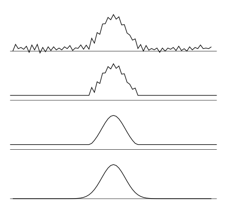
When estimating sums across the whole range, we want to take advantage of our ability to get accurate estimates of the summand in various different parts of the range. On the other hand, it is certainly more convenient if we can stick to a single function across the entire range of interest. In this section, we discuss a general method that allows us to do both, the Laplace method for estimating the value of sums and integrals. We frequently encounter sums in the analysis of algorithms that can be estimated with this approach. Generally, we are also taking advantage of our ability to approximate sums with integrals in such cases. The method is centered around the following three steps for evaluating sums:- Restrict the range to an area that contains the largest summands.
- Approximate the summand and bound the tails.
- Extend the range and bound the new tails, to get a simpler sum.
This figure illustrates the method in a schematic manner. Actually, when approximating sums, the functions involved are all step functions; usually a “smooth” function makes an appearance at the end, in an application of the Euler-Maclaurin formula.
Example (Ramanujan Q-function). To approximate $$Q(N)\equiv\sum_{1\le k\le N} {N!\over (N-k)!N^k}$$ apply the approximations just given to different ranges of the sum. More precisely, define $k_0$ to be an integer that is $o(N^{2/3})$ and divide the sum into two parts: $$\sum_{1\le k\le N} {N!\over (N-k)!N^k} = \sum_{1\le k\le k_0} {N!\over (N-k)!N^k} + \sum_{k_0 < k\le N} {N!\over (N-k)!N^k}.$$ We approximate the two parts separately, using the different restrictions on $k$ in the two parts to advantage. For the first (main) term, we use the uniform approximation. For the second term (the tail), the restriction $k>k_0$ and the fact that the terms are decreasing imply that they are all exponentially small. $$Q(N)=\sum_{1\le k\le k_0} e^{-k^2/(2N)}\Bigl(1 + O({k\over N})+ O({k^3\over N^2})\Bigr)+\Delta.$$ Here we use $\Delta$ as a notation to represent a term that is exponentially small, but otherwise unspecified. The main term $\exp(-k^2/(2N)$ is also exponentially small for $k>k_0$ and we can add the terms for $k>k_0$ back in, so we have $$Q(N)\,=\,\sum_{k\ge1}\,\,\,e^{-k^2/(2N)} + O(1).$$ Essentially, we have replaced the tail of the original sum by the tail of the approximation, which is justified because both are exponentially small. The remaining sum is the sum of values of the function $e^{x^2/2}$ at regularly spaced points with step $1/\sqrt{N}$. Thus, the Euler-Maclaurin theorem provides the approximation $$\sum_{k\ge1}e^{-k^2/(2N)}=\sqrt{N}\int_0^\infty e^{-{x^2/2}}dx + O(1).$$ The value of this integral is well known to be $\sqrt{\pi/2}$. Substituting into the above expression for $Q(N)$ gives the result $$Q(N) = \sqrt{\pi N/2} +O(1).$$
4.8 "Normal" Examples from the Analysis of Algorithms
4.9 "Poisson" Examples from the Analysis of Algorithms
4.10 Generating Function Asymptotics
Selected Exercises
4.2
Show that $$\displaystyle{N\over N+1}=1+O\Bigl({1\over N}\Bigr)\qquad\hbox{and}\qquad \displaystyle{N\over N+1}\sim 1-{1\over N}.$$4.9
If $\alpha<\beta$, show that $\alpha^N$ is exponentially small relative to $\beta^N$. You may use that fact that $e^{-N\epsilon}$ is exponentially small for any $\epsilon > 0$. For $\beta=1.2$ and $\alpha=1.1$, find the absolute and relative errors when $\alpha^N+\beta^N$ is approximated by $\beta^N$, for $N=10$ and $N=100$.4.14
Use Theorem 4.1 to find an asymptotic solution to the recurrence $$a_n=5a_{n-1}-8a_{n-2}+4a_{n-3}\qquad\hbox{for $n>2$ with $a_0=1$, $a_1=2$, and $a_2=4$}.$$ Solve the same recurrence with the initial conditions on $a_0$ and $a_1$ changed to $a_0=1$ and $a_1=2$.4.15
Use Theorem 4.1 to find an asymptotic solution to the recurrence $$a_n=2a_{n-2}-a_{n-4}\qquad\hbox{for $n>4$ with $a_0=a_1=0$ and $a_2=a_3=1$}.\ $$4.16
Use Theorem 4.1 to find an asymptotic solution to the recurrence $$a_n=3a_{n-1}-3a_{n-2}+a_{n-3}\qquad\hbox{for $n>2$ with $a_0=a_1=0$ and $a_2\ =1$}.$$4.21
Expand $\ln(1-x+x^2)$ as $x\to0$, to within $O\bigl(x^4\bigr)$.4.23
Give an asymptotic expansion for $\displaystyle{N\over N-1}\ln {N\over N-1}$ to within $\displaystyle O\bigl({1\over N^4}\bigr)$.4.38
Calculate an asymptotic expansion for $(3N)!/(N!)^3$ to within relative precision $\displaystyle\Bigl(1+ O({1\over N})\Bigr)$.4.39
What is the approximate value of $\displaystyle\Bigl(1-{\lambda\over N}\Bigr)^N$?4.50
Give an asymptotic estimate for $\sum_{0\le k\le N}{2^k/(2^k+1)}$.4.58
Use Euler-Maclaurin summation to estimate $$\sum_{1\le k\le N}{\sqrt{k}},\qquad \sum_{1\le k\le N}{1\over\sqrt{k}},\quad\hbox{and}\quad \sum_{1\le k\le N}{1\over\root3\of{k}}$$ to within $O\bigl(1/N^2\bigr)$.4.71
Show that ${(N-k)^k(N-k)!\over N!} = e^{ - {k^2\over 2N}}\Bigl( 1 + O({k\over N}) + O({k^3\over N^2})\Bigr) $ for $k = o(N^{2/3})$. By the same arguments as in the proofs of Theorems 4.5, 4.8, and the Corollary to Theorem 4.4, you could extend this derivation to prove that $$ P(N)=\sum_{0\le k < N} {(N-k)^k(N-k)!\over N!}=\sqrt{\pi N/2}+O(1)$$