


6. Trees
This chapter investigates properties of many different types of
trees, fundamental structures that arise implicitly and explicitly
in many practical algorithms. Our goal is to provide access to results
from an extensive literature on the combinatorial analysis of trees,
while at the same time providing the groundwork for a host of
algorithmic applications.
6.1 Binary Trees
Definition. A binary tree is either an external node or an internal node attached to an ordered pair of binary trees called the left subtree and the right subtree of that node.
Theorem. (Enumeration of binary trees) The number of binary trees with $N$ internal nodes and $N+1$ external nodes is given by the Catalan numbers: $$T_{N}={1\over N+1}{2N\choose N} = {4^N\over\sqrt{\pi N^3}}\Bigl(1+O({1\over N})\Bigr).$$ Proof.
6.2 Forests and Trees
In a binary tree, no node has more than two children. This characteristic makes it obvious how to represent and manipulate such trees in computer implementations, and it relates naturally to “divide-and-conquer” algorithms that divide a problem into two subproblems. However, in many applications (and in more traditional mathematical usage), we need to consider general trees:Definition. A tree (also called a general tree) is a node (called the root) connected to a sequence of disjoint trees. Such a sequence is called a forest.
We use the same nomenclature as for binary trees: the subtrees of a node are its children, a root node has no parents, and so forth. Trees are more appropriate models than binary trees for certain computations.
Theorem. (Enumeration of general trees) Let $G_N$ be the number of general trees with $N$ nodes. Then $G_N$ is exactly equal to the number of binary trees with $N-1$ internal nodes and is given by the Catalan numbers: $$G_N=T_{N-1}={1\over N}{2N-2\choose N-1}.$$ Proof. (via the symbolic method) A forest is either empty or a sequence of trees: $$\cal F = \epsilon + \cal G + (\cal G\times\cal G) + (\cal G\times\cal G\times\cal G) + (\cal G\times\cal G\times\cal G\times\cal G) + \ldots$$ which translates directly to $$F(z) = 1 + G(z) + G(z)^2 + G(z)^3 + G(z)^4 + \ldots = {1\over 1-G(z)}.$$ The obvious one-to-one correspondence between forests and trees (cut off the root) means that $zF(z) = G(z)$, so $$G(z)={z\over 1-G(z)}.$$ Thus $G(z)-G(z)^2=z$ and therefore $G(z)=zT(z)$, since both functions satisfy the same functional equation. That is, the number of trees with $N$ nodes is equal to the number of binary trees with $N$ external nodes.
6.3 Combinatorial Equivalences to Trees and Binary Trees
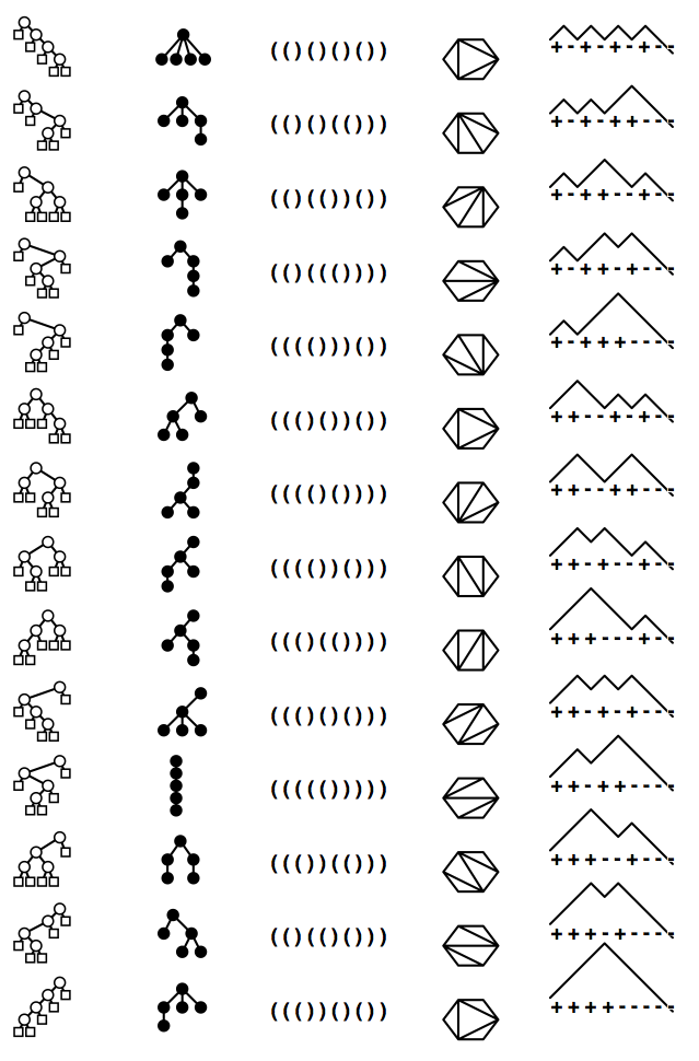
The following combinatorial objects are all in 1-1 correspondence and are therefore counted by the Catalan numbers.- Binary trees with $N$ external nodes.
- Trees with $N$ nodes.
- Legal sequences of $N$ pairs of parentheses.
- Triangulated $N$-gons.
- Gambler's ruin sequences.
Here are examples of these objects for small $N$:
6.4 Properties of Trees
Definition. In a tree $t$:
- the size $|t|$ is its number of nodes
- the level of a node is its distance from the root (which is at level 0)
- the path length $\pi(t)$ is the sum of the levels of each of the nodes in $t$
- the height $\eta(t)$ is the maximum level among all the nodes
- the leaves are the nodes with no children
- the size $|t|$ is its number of internal nodes
- the level of a node is its distance from the root (which is at level 0)
- the internal path length $\pi(t)$ is the sum of the levels of each of the internal nodes in $t$
- the external path length $\xi(t)$ is the sum of the levels of each of the external nodes in $t$
- the height $\eta(t)$ is the maximum level among all the external nodes
- the leaves are the (internal) nodes with both children external
In the analysis of algorithms, we are particularly interested in knowing the average values of these parameters, for various types of “random” trees. One of our primary topics of discussion for this chapter is how these quantities relate to fundamental algorithms and how we can determine their expected values. A random binary tree has larger values for both path length and height than a random forest. One of the prime objectives of this chapter is to quantify these and similar observations, precisely.Example. Path lengths in any binary tree $t$ satisfy $\xi({t})=\pi({t})+2|t|$. Subtracting the equation $\pi(t)=\pi(t_l)+\pi(t_r)+|t|-1$ from the equation $\xi(t)=\xi(t_l)+\xi(t_r)+|t|+1$ immediately provides the basis for a proof by induction.
6.5 Examples of Tree Algorithms
Trees are relevant to the study of analysis of algorithms not only
because they implicitly model the behavior of recursive programs
but also because they are involved explicitly in many basic algorithms
that are widely used. For typical applications, we are interested in the path
length and height of trees. To consider the average value of
such parameters, of course, we need to specify a model defining what
is meant by a random tree. For
applications such as tree traversal and
expression evaluation
(or, more generally,
recursive program execution,
the model where trees are taken equally likely is worth considering.
For these applications, we study
so-called Catalan models, where each of the
$T_N$ binary trees of size $N$ or general trees of size $N+1$ are taken with
equal probability. This is not the only possibility---in many situations,
the trees are induced by external data, and other models
of randomness are appropriate. Next, we consider a particularly important
example.
6.6 Binary Search Trees
One of the most important applications of binary trees is the binary tree search algorithm, a method that uses binary trees explicitly to provide an efficient solution to a fundamental problem in computer science. For full details, see Section 3.2 in Algorithms, 4th edition. The analysis of binary tree search illustrates the distinction between models where all trees are equally likely to occur and models where the underlying distribution is nonuniform. The juxtaposition of these two is one of the essential concepts of this chapter.Definition. A binary search tree is a binary tree with keys associated with the internal nodes, satisfying the constraint that the key in every node is greater than or equal to all the keys in its left subtree and less than or equal to all the keys in its right subtree.
We study binary search trees under the random permutation model, where we assume that each permutation of the keys in the tree (all distinct) is equally likely as input. This model has been validated in many practical situations. Many different permutations may map to the same tree. It is not true that each tree is equally likely to occur if keys are inserted in random order into an initially empty tree.
The cost of constructing a particular tree is directly proportional to its internal path length, since nodes are not moved once inserted, and the level of a node is exactly the number of nodes required to insert it. Thus, the cost of constructing a tree is the same for each of the permutations that could lead to its construction.
We could obtain the average construction cost by adding, for all $N!$ permutations, the internal path length of the resulting tree (the cumulated cost) and then dividing by $N!$. The cumulated cost also could be computed by adding, for all trees, the product of the internal path length and the number of permutations that lead to the tree being constructed. This is the average internal path length that we expect after $N$ random insertions into an initially empty tree, but it is not the same as the average internal path length of a random binary tree, under the Catalan model where all trees are equally likely. It requires a separate analysis. We will consider the Catalan tree case in the next section and the binary search tree case in Section 6.8. Indeed, it is fortunately the case that the more balanced tree structures, for which search and construction costs are low, are more likely to occur than tree structures for which the costs are high. In the analysis, we will quantify this.
6.7 Average Path Length in Catalan Trees
What is the average path length of a tree with $N$ internal nodes, if each $N$-node tree is considered to be equally likely? Our analysis of this important question is prototypical of the general approach to analyzing parameters of combinatorial structures that we introduced in Chapter 3:- Define a bivariate generating function (BGF), with one variable marking the size of the tree and the other marking the internal path length.
- Derive a functional equation satisfied by the BGF, or its associated cumulative generating function (CGF).
- Extract coefficients to derive the result.
In a random binary Catalan tree with $N$ nodes,
the probability that the left subtree has
$k$ nodes (and the right subtree has $N-k-1$ nodes) is
$T_{k}T_{N-k-1}/T_N$ (where $T_N={2N\choose N}\bigm / (N+1)$
is the $N$th Catalan number).
The denominator is the number of possible $N$-node trees and the
numerator counts the number of ways to make an $N$-node tree by
using any tree with $k$ nodes on the left and any tree with $N-k-1$
nodes on the right. We refer to this probability distribution as
the Catalan distribution, illustrated in this figure.
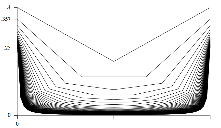
One of the striking facts about the distribution is that
the probability that one of the subtrees is empty tends to
a constant as $N$ grows: it is $2T_{N-1}/T_N\sim 1/2$. Indeed, about half
the nodes in a random binary tree are likely to have an empty subtree,
so such trees are not particularly well balanced.
Using the Catalan distribution, we can analyze path length
in a manner similar to our Quicksort analysis.
The average internal
path length in a random binary Catalan tree is described
by the recurrence
$$Q_N=N-1+\sum_{1\le k\le N}{T_{k-1}T_{N-k}\over T_N}(Q_{k-1}+Q_{N-k})
\qquad\hbox{for $N>0$}
$$
with $Q_0=0$.
The argument underlying this recurrence is general, and can be used to
analyze random binary tree structures under other models of randomness,
by substituting other distributions for the Catalan distribution.
For example, as discussed below, the analysis
of binary search trees leads to the uniform
distribution (each subtree size occurs with probability $1/N$) and the
recurrence matches the Quicksort recurrence. Continuing along the lines
of the Quicksort analysis is possible but leads to intricate calculations,
easily avoided with CGFs.
Theorem. (Path length in binary trees) The average internal path length in a random binary tree with $N$ internal nodes is $${(N+1)4^N\over{2N\choose N}}-3N-1 = N\sqrt{\pi N}-3N+O(\sqrt{N}).$$ Proof. Define the CGF $$C_T(z) \equiv P_u(1,z) = \sum_{t\in \cal T}\pi(t)z^{|t|}.$$ The average path length is $[z^n]C_T(z)/[z^n]T(z)$. The recursive definition of binary trees leads immediately to $$\eqalign{C_T(z) &= \sum_{t_l\in \cal T}\sum_{t_r\in\cal T} (\pi(t_l ) + \pi(t_r ) + |t_l | + | t_r|) z^{|t_l| + |t_r| + 1}\cr &= 2zC_T(z)T(z)+2z^2T(z)T^\prime(z),\cr} $$ which yields the solution $$C_T(z) = {2z^2T(z)T^\prime(z)\over 1-2zT(z)}.$$ Now, $T(z)=(1-\sqrt{1-4z})/(2z)$, so $1-2zT(z)=\sqrt{1-4z}$ and $zT^\prime(z)=-T(z)+1/\sqrt{1-4z}$. Substituting these gives the explicit expression $$zC_T(z) = {z \over 1-4z} - {1 -z\over \sqrt {1-4z}} + 1,$$ which expands to give the stated result.
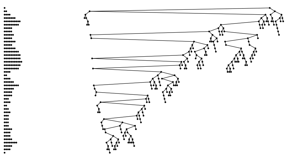
This result is illustrated by the large random binary tree shown below:
asymptotically, a large tree roughly fits into a $\sqrt{N}$-by-$\sqrt{N}$
square.
Theorem. (Path length in general trees) The average path length in a random general tree with $N$ internal nodes is $${N\over 2}\biggl({4^{N-1}\over{2N-2\choose N-1}}-1\biggr) = {N\over2}\bigl(\sqrt{\pi N}-1\bigr)+O({\sqrt{N}}).$$ Proof. Proceed as above: $$\eqalign{ C_G(z)&\equiv\sum_{t\in\cal G}{\pi(t)}z^{|t|}\cr &=\sum_{k\ge0}\sum_{t_1\in\cal G}\dots\sum_{t_k\in\cal G} (\pi(t_1)+\cdots+\pi(t_k)+|t_1|+\ldots+|t_k|) z^{|t_1|+\ldots+|t_k|+1}\cr }$$ This (eventually) leads to the equation $$C_G(z) = {zC_G(z)+z^2G^\prime(z)\over(1-G(z))^2}.$$ which simplifies to give $$C_G(z)={1\over2}{z\over1-4z}-{1\over2}{z\over\sqrt{1-4z}}.$$ where $G(z)=zT(z)=(1-\sqrt{1-4z})/2$ is the Catalan generating function, which enumerates general trees. Expanding $[z^N]C_G(z)/[z^N]G(z)$ leads to the stated result.
6.8 Path Length in Binary Search Trees
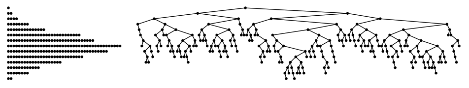
The analysis of path length in binary search trees is actually the study of a property of permutations, not trees, since we start with a random permutation. In Chapter 7, we discuss properties of permutations as combinatorial objects in some detail. We mention the analysis of path length in BSTs here not only because it is interesting to compare it with the analysis just given for random trees. It is virtually identical to our Quicksort analysis.Theorem. (Construction cost of BSTs.) The average number of comparisons involved in the process of constructing a binary search tree by inserting $N$ distinct keys in random order into an initially empty tree (the average internal path length of a random binary search tree) is $$2(N+1)(H_{N+1}-1)-2N\approx 1.386 N\lg N - 2.846 N$$ with variance asymptotic to $(7-2\pi^2/3)N^2$.
Asymptotically, a large BST roughly fits into a $\log{N}$-by-$N/\log{N}$
rectangle.
6.9 Additive Parameters of Random Trees.
Our analyses for path length generalize in a straightforward manner to cover any additive parameter that can be aligned with the tree recursion as follows: the value of the parameter for a tree is the sum of the values of the parameter for the subtrees plus an additional term for the root. Examples of additive parameters include size, path length, and number of leaves.
6.10 Height
Generating functions can also be used to study tree height, but the analysis is much more intricate than for additive parameters.
6.11 Summary of Average-Case Results on Properties of Trees
| type | path length | height | leaves |
|---|---|---|---|
| tree | $${N\over 2}\sqrt{\pi N} -{N\over 2}+ O(\sqrt{N})$$ | $$\sqrt{\pi N} +O(1)$$ | $$N\over2$$ |
| binary tree | $$N\sqrt{\pi N}-3N+O(\sqrt{N})$$ | $$2\sqrt{\pi N} +O(N^{1/4 + \epsilon})$$ | $$\sim{N\over4}$$ |
| BST | $$2N\ln N+(2\gamma-4)N+O(\log N)$$ | $$\sim 4.31107...\ln N$$ | $$\qquad {N+1\over3}\qquad$$ |
6.12 Lagrange Inversion
6.13 Rooted Unordered Trees
The following are four major types of trees that arise in the analysis of algorithms, which form a hierarchy:- The free tree, an acyclic connected graph.
- The rooted tree, a free tree with a distinguished root node.
- The ordered tree, a rooted tree where the order of the subtrees of a node is significant.
- The binary tree is an ordered tree where every node has degree 0 or 2.
In the nomenclature that we use, the adjective describes the characteristic
that separates each type of tree from the one above it in the hierarchy.
It is also common to use nomenclature that separates each type
from the one below it in the hierarchy. Thus, we sometimes
refer to free trees as unrooted trees, rooted trees as unordered trees,
and ordered trees as general Catalan trees.
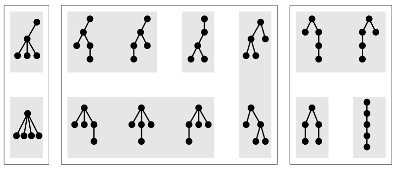
Here is an illustration of the hierarchy for trees with five nodes.
The 14 different five-node ordered trees are depicted in the figure,
and they are further organized into equivalence classes using small
shaded and larger open rectangles. There are 9 different five-node rooted
trees (those in shaded rectangles are identical as
rooted trees) and 3 different five-node free trees
(those enclosed in large rectangles are identical as free trees).
A few more words on nomenclature are appropriate because of the
variety of terms found in the literature. Ordered trees are often
called plane trees and unordered trees are referred to as
nonplane trees. The term plane is used because the
structures can be transformed to one another with continuous
operations in the plane. Though this terminology is widely used, we
prefer ordered because of its natural implications with regard to
computer representations. The term oriented is often used
to refer to the fact
that the root is distinguished, so there is an orientation of the
edges towards the root; we prefer to use the term rooted if it is
not obvious from the context that there is a root involved.
As the definitions get more restrictive, the number of trees
that are regarded as different gets larger, so, for a given size,
there are more rooted trees than free trees, more ordered trees than
rooted trees, and more binary trees than ordered trees. It turns out
that the ratio between the number of rooted trees and the number of
free trees is proportional to $N$; the corresponding ratio of ordered
trees to rooted trees grows exponentially with $N$; and the ratio of
binary trees to ordered trees is a constant. These enumerations
results are classical, available through analysis along the lines we
have been considering (we considered the analysis for ordered
and binary trees earlier in this chapter)
and summarized in the table below. The constants
in the table are approximate and $\alpha\approx 2.9558$.
| type | number of trees with N nodes |
|---|---|
| free | $$\sim .5350\cdot\alpha^N / N^{5/2}$$ |
| rooted | $$\sim .4399\cdot\alpha^N / N^{3/2}$$ |
| ordered | $$\sim .1410\cdot 4^N / N^{3/2}$$ |
| binary | $$\sim .5640\cdot 4^N N^{3/2}$$ |
6.14 Labelled Trees
6.15 Other Types of Trees
It is often convenient to place various local and global restrictions on trees, for example, to suit requirements of a particular application or to try rule out degenerate cases. From a combinatorial standpoint, any restriction corresponds to a new class of tree, and a new set of problems need to be solved to enumerate the trees and to learn their statistical properties.
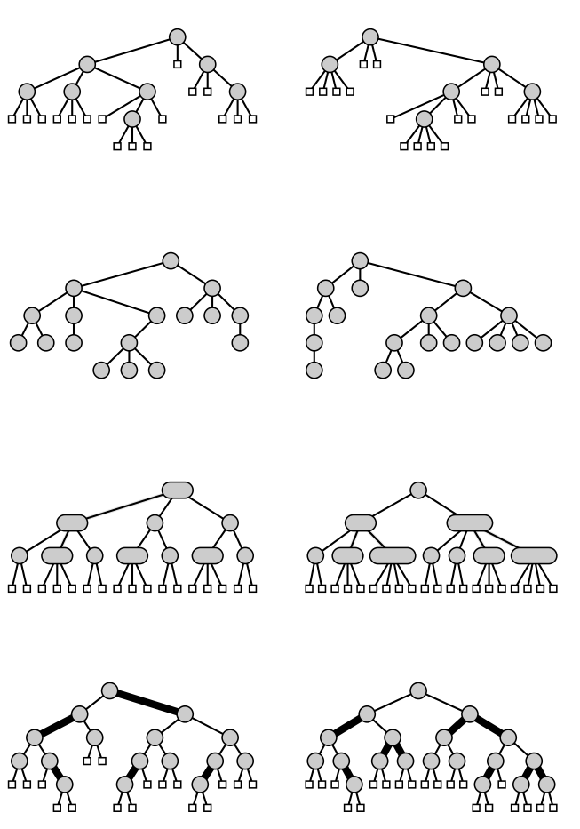
This table shows examples of eight different types of trees:
3-ary and 4-ary, 3-restricted and 4-restricted, 2-3 and 2-3-4, and
red-black and AVL.
Selected Exercises
6.2
What proportion of the binary trees with $N$ internal nodes have both subtrees of the root nonempty? For $N=4$, the answer is $4/14$.6.6
What proportion of the forests with $N$ nodes have no trees consisting of a single node? For $N=1,2,3,$ and $4$, the answers are $0, 1/2, 2/5,$ and $3/7$, respectively6.18
[Kraft equality] Let $k_j$ be the number of external nodes at level $j$ in a binary tree. The sequence $\{ k_0, k_1, \ldots, k_h \}$ (where $h$ is the height of the tree) describes the profile of the tree. Show that a vector of integers describes the profile of a binary tree if and only if $\sum_j2^{-k_j} = 1$.6.19
Give tight upper and lower bounds on the path length of a general tree with $N$ nodes.6.20
Give tight upper and lower bounds on the internal and external path lengths of a binary tree with $N$ internal nodes.6.27
For $N=2^n-1$, what is the probability that a perfectly balanced tree structure (all $2^n$ external nodes on level $n$) will be built, if all $N!$ key insertion sequences are equally likely?6.42
Internal nodes in binary trees fall into one of three classes: they have either two, one, or zero external children. What fraction of the nodes are of each type, in a random binary Catalan tree of $N$ nodes?6.43
Internal nodes in binary trees fall into one of three classes: they have either two, one, or zero external children. What fraction of the nodes are of each type, in a random binary search tree of $N$ nodes?
Review Questions
Q6.1
Give an asymptotic approximation (leading term) for the number of unary-binary trees with $n$ nodes.Q6.2
Rank these trees in order of their likely height for large $n$: (a) random $n$_node Catalan tree (b) random $n$_node BST (c) random $n$_node AVL treeQ6.3
A binary trie structure is a binary tree with two types of external nodes (void and nonvoid) with the restriction that void external nodes do not appear in leaves. The number of different binary trie structures with n external nodes is 1, 4, and 17 when n is 2, 3, and 4, respectively. Starting with the construction $$T = Z_V+(Z_I\times T\times T)+2(Z_N\times Z_I\times (T - Z_V)) $$ derive an asymptotic approximation to the number of binary trie structures of with n external nodes.
Hint: $$\sqrt{12z^2-8z+1} = {\sqrt{1-2z}\over(1-6z)^{-1/2}}$$.